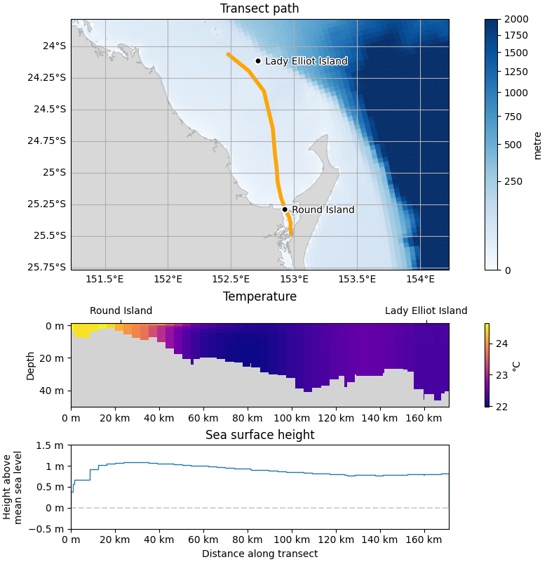
K’gari transect plot

import shapely
import matplotlib.pyplot as plt
from matplotlib import gridspec
from matplotlib.colors import LogNorm, PowerNorm

import emsarray
from emsarray import plot, transect, utils
from emsarray.operations import depth

dataset_url = 'https://thredds.nci.org.au/thredds/dodsC/fx3/gbr4_H4p0_ABARRAr2_OBRAN2020_FG2Gv3_Dhnd/gbr4_simple_2022-10-01.nc'
# dataset_url = '~/example-datasets/gbr4_simple_2022-10-31.nc'
dataset = emsarray.open_dataset(dataset_url).isel(time=12)
# Select only the variables we want to plot.
dataset = dataset.ems.select_variables(['botz', 'temp', 'eta'])
# The depth coordinate has positive=up, while the bathymetry has positive=down.
# This causes issues when drawing the ocean floor.
# Lets fix the depth coordinate.
dataset = depth.normalize_depth_variables(dataset, ['zc'], positive_down=True)
# Cross section plots need bounds information, so lets invent some
dataset = utils.estimate_bounds_1d(dataset, 'zc')

The following is a transect path starting in the Great Sandy Strait near K’gari, heading roughly North out to deeper waters:

north_transect = transect.Transect(dataset, shapely.LineString([
    [152.9768944, -25.4827962],
    [152.9701996, -25.4420345],
    [152.9727745, -25.3967620],
    [152.9623032, -25.3517828],
    [152.9401588, -25.3103560],
    [152.9173279, -25.2538563],
    [152.8962135, -25.1942238],
    [152.8692627, -25.0706729],
    [152.8623962, -24.9698750],
    [152.8472900, -24.8415806],
    [152.8308105, -24.6470172],
    [152.7607727, -24.3521012],
    [152.6392365, -24.1906056],
    [152.4792480, -24.0615124],
]))
landmarks = [
    ('Round Island', shapely.Point(152.9262543, -25.2878719)),
    ('Lady Elliot Island', shapely.Point(152.7145958, -24.1129146)),
]

Set up three axes: one showing the transect path, one showing a temperature cross section along the transect, and one showing the sea surface height along the transect.

figure = plt.figure(figsize=(7.8, 8), layout='constrained', dpi=100)
gs_root = gridspec.GridSpec(3, 1, figure=figure, height_ratios=[3, 1, 1])
path_axes = figure.add_subplot(gs_root[0], projection=dataset.ems.data_crs)
temp_axes = figure.add_subplot(gs_root[1])
eta_axes = figure.add_subplot(gs_root[2], sharex=temp_axes)

First make a plot showing the path of the transect overlayed on the bathymetry

path_axes.set_aspect(aspect='equal', adjustable='datalim')
path_axes.set_title('Transect path')
dataset.ems.make_artist(
    path_axes, 'botz', cmap='Blues', clim=(0, 2000), edgecolor='face',
    norm=PowerNorm(gamma=0.5),
    linewidth=0.5, zorder=0)
path_axes.set_extent(plot.bounds_to_extent(north_transect.line.envelope.buffer(0.2).bounds))
path_axes.plot(*north_transect.line.coords.xy, zorder=1, c='orange', linewidth=4)

plot.add_coast(path_axes, zorder=1)
plot.add_gridlines(path_axes)
plot.add_landmarks(path_axes, landmarks)

Now plot a cross section along the transect showing the ocean temperature. As the temperature variable has a depth axis the cross section is two dimensional.

temp_axes.set_title('Temperature')
dataset['temp'].attrs['units'] = '°C'
dataset['zc'].attrs['long_name'] = 'Depth'

north_transect.make_artist(
    temp_axes, 'temp', cmap='plasma')
north_transect.make_ocean_floor_artist(
    temp_axes, dataset['botz'])
# yaxis
transect.setup_depth_axis(
    north_transect, temp_axes, data_array='temp',
    label='Depth', ylim=(50, -1.5))

Now plot the sea surface height along the transect. As the sea surface height does not have a depth axis the transect is one dimensional.

eta_axes.set_title('Sea surface height')
eta_artist = north_transect.make_artist(
    eta_axes, data_array=dataset['eta'])
# xaxis
transect.setup_distance_axis(north_transect, eta_axes)
# yaxis
eta_axes.set_ylim(-0.5, 1.5)
eta_axes.set_ylabel('Height above\nmean sea level')
eta_axes.axhline(0, linestyle='--', color='lightgrey')
eta_axes.yaxis.set_major_formatter("{x:.2g} m")

The last step is to add some landmarks along the top border of the axes to help viewers link the distance along transect path to geographic locations.

top_axis = temp_axes.secondary_xaxis('top')
top_axis.set_ticks(
    [north_transect.distance_along_line(point) for label, point in landmarks],
    [label for label, point in landmarks],
)


plt.show()