Plotting
Contents
Plotting#
emsarray can produce simple plots, to help you visualise your data quickly. Plots can be made from any supported format.
[1]:
import emsarray
Set up the environment…
[2]:
# This makes the figures nice and big for this notebook
from matplotlib import pyplot as plt
plt.rcParams['figure.dpi'] = 100
plt.rcParams['figure.figsize'] = (8, 5)
plt.rcParams['savefig.dpi'] = 100

# The coastlines used in the maps have some bad polygons,
# which cause some warnings. Lets turn those off.
import warnings
warnings.filterwarnings(
    "ignore", message="Shapefile shape has invalid polygon",
    category=UserWarning, module="shapefile")
A quick demonstration before we get started!
[3]:
gbr4 = emsarray.tutorial.open_dataset('gbr4')
gbr4
[3]:
<xarray.Dataset>
Dimensions:    (k: 47, j: 180, i: 600, time: 1)
Coordinates:
    zc         (k) float32 -3.89e+03 -3.68e+03 -3.48e+03 ... -0.5 0.5 1.5
    longitude  (j, i) float32 ...
    latitude   (j, i) float32 ...
  * time       (time) datetime64[ns] 2022-05-11T14:00:00
Dimensions without coordinates: k, j, i
Data variables:
    botz       (j, i) float32 ...
    eta        (time, j, i) float32 ...
    salt       (time, k, j, i) float32 ...
    temp       (time, k, j, i) float32 ...
Attributes: (12/14)
    title:                           GBR4 Hydro
    description:                     New eReefs GBR 4k grid with rivers. Uses...
    paramhead:                       GBR 4km resolution grid
    paramfile:                       ./prm/gbr4_hydro_nrt.prm
    ems_version:                     v1.4.0 rev(6949)
    date_created:                    Mon May 16 09:30:33 2022
    ...                              ...
    Run_code:                        GBR4 Hydro|G0.00|H2.10|S0.00|B0.00
    Parameter_File_Revision:         $Revision: 1753 $
    bald__isPrefixedBy:              prefix_list
    prefix_list_puv__:               https://w3id.org/env/puv#
    prefix_list_qudt__:              http://qudt.org/vocab/unit/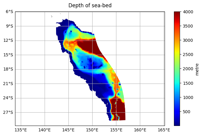
DODS_EXTRA.Unlimited_Dimension: timeThe botz variable indicates the depth of the ocean floor at a particular cell.
The data will be plotted on a map, wih coastlines overlayed. A colour ramp will be applied and automatically scaled to the range of the data.
[4]:
gbr4.ems.plot('botz', title='Depth of sea-bed')
Selecting what to plot#
A plot has to be made of a single layer. For datasets with multiple depth layers and multiple time steps, start by selecting just one slice from each of these extra dimensions.
The BRAN2020 example file contains multiple time steps and multiple depth layers. We will need to select just one of each before we can make a plot.
[5]:
bran2020 = emsarray.tutorial.open_dataset('bran2020')
bran2020
[5]:
<xarray.Dataset>
Dimensions:   (xt_ocean: 100, yt_ocean: 100, st_ocean: 30, Time: 20, nv: 2)
Coordinates:
  * xt_ocean  (xt_ocean) float64 140.1 140.1 140.2 140.4 ... 149.8 149.9 149.9
  * yt_ocean  (yt_ocean) float64 -46.95 -46.85 -46.75 ... -37.25 -37.15 -37.05
  * st_ocean  (st_ocean) float64 2.5 7.5 12.5 17.52 ... 233.2 255.9 286.6 325.9
  * Time      (Time) datetime64[ns] 2021-12-01T12:00:00 ... 2021-12-20T12:00:00
  * nv        (nv) float64 1.0 2.0
Data variables:
    temp      (Time, st_ocean, yt_ocean, xt_ocean) float32 ...
Attributes:
    filename:                        TMP/ocean_temp_2021_12_01.nc.0000
    NumFilesInSet:                   20
    grid_type:                       regular
    grid_tile:                       N/A
    history:                         Fri Feb 11 09:56:43 2022: ncrcat -4 --df...
    NCO:                             netCDF Operators version 5.0.5 (Homepage...
    title:                           BRAN2020
    catalogue_doi_url:               http://dx.doi.org/10.25914/6009627c7af03
    acknowledgement:                 BRAN is made freely available by CSIRO B...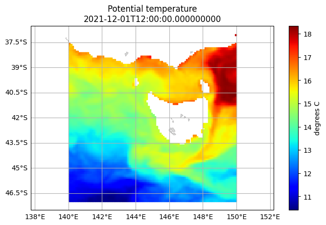
DODS_EXTRA.Unlimited_Dimension: TimeUsing dataset.isel(...) we can trim the data so we have just the surface layer at the first timestep. After that we plot the temp variable:
[6]:
bran2020.isel(Time=0, st_ocean=0).ems.plot('temp')
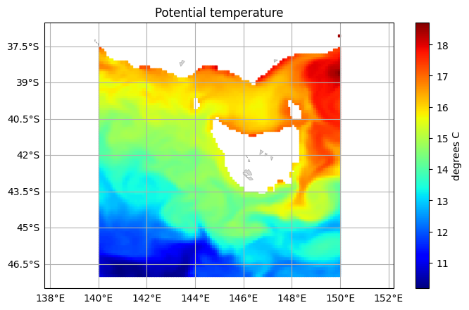
Instead of selecting a subset of the data across the entire dataset, you can slice a single data array and plot that variable directly. To demonstrate, we can plot the last time step by selecting it on the data array:
[7]:
temp = bran2020['temp'].isel(Time=-1, st_ocean=0)
bran2020.ems.plot(temp)
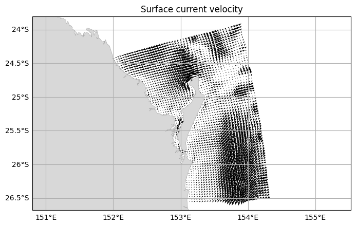
Plotting vectors#
You can plot vector data using two variables that make up the u and v components of the vector.
[8]:
fraser = emsarray.tutorial.open_dataset('fraser')
fraser
[8]:
<xarray.Dataset>
Dimensions:    (k: 47, j: 50, i: 70, time: 24)
Coordinates:
    zc         (k) float32 -3.89e+03 -3.68e+03 -3.48e+03 ... -0.5 0.5 1.5
    longitude  (j, i) float32 152.0 152.0 152.0 152.1 ... 154.3 154.3 154.3
    latitude   (j, i) float32 -24.43 -24.46 -24.49 ... -26.41 -26.44 -26.48
  * time       (time) datetime64[ns] 2022-05-11T14:00:00 ... 2022-05-12T12:59...
Dimensions without coordinates: k, j, i
Data variables:
    botz       (j, i) float32 5.43 4.47 3.23 nan nan ... 4e+03 4e+03 4e+03 4e+03
    eta        (time, j, i) float32 -0.4719 -0.4735 -0.4707 ... -0.4622 -0.4597
    u          (time, k, j, i) float32 ...
    v          (time, k, j, i) float32 ...
    temp       (time, k, j, i) float32 ...
Attributes: (12/14)
    title:                           GBR4 Hydro
    description:                     New eReefs GBR 4k grid with rivers. Uses...
    paramhead:                       GBR 4km resolution grid
    paramfile:                       ./prm/gbr4_hydro_nrt.prm
    ems_version:                     v1.4.0 rev(6949)
    date_created:                    Mon May 16 09:30:33 2022
    ...                              ...
    Run_code:                        GBR4 Hydro|G0.00|H2.10|S0.00|B0.00
    Parameter_File_Revision:         $Revision: 1753 $
    bald__isPrefixedBy:              prefix_list
    prefix_list_puv__:               https://w3id.org/env/puv#
    prefix_list_qudt__:              http://qudt.org/vocab/unit/
DODS_EXTRA.Unlimited_Dimension: time[9]:
# Select the surface currents at the first timestep
fraser_0 = fraser.isel(time=0, k=-1)

fraser.ems.plot(
    vector=(fraser_0["u"], fraser_0["v"]),
    title="Surface current velocity")
/home/docs/checkouts/readthedocs.org/user_builds/emsarray/conda/v0.1.0/lib/python3.9/site-packages/cartopy/io/__init__.py:241: DownloadWarning: Downloading: https://www.ngdc.noaa.gov/mgg/shorelines/data/gshhs/latest/gshhg-shp-2.3.7.zip
  warnings.warn(f'Downloading: {url}', DownloadWarning)
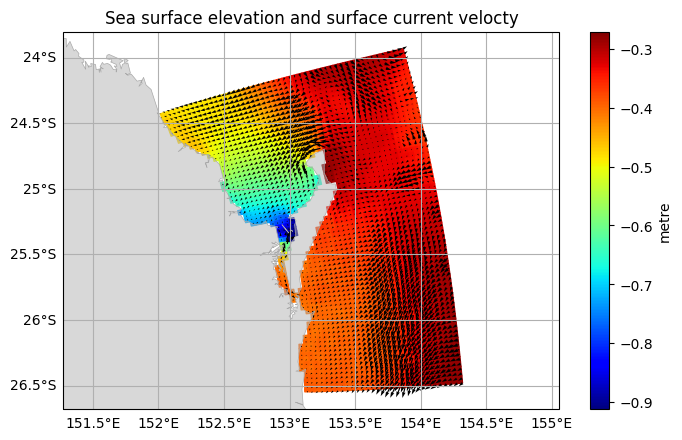
This can be combined with a scalar plot:
[10]:
fraser.ems.plot(
    scalar=fraser_0["eta"],
    vector=(fraser_0["u"], fraser_0["v"]),
    title="Sea surface elevation and surface current velocty",)
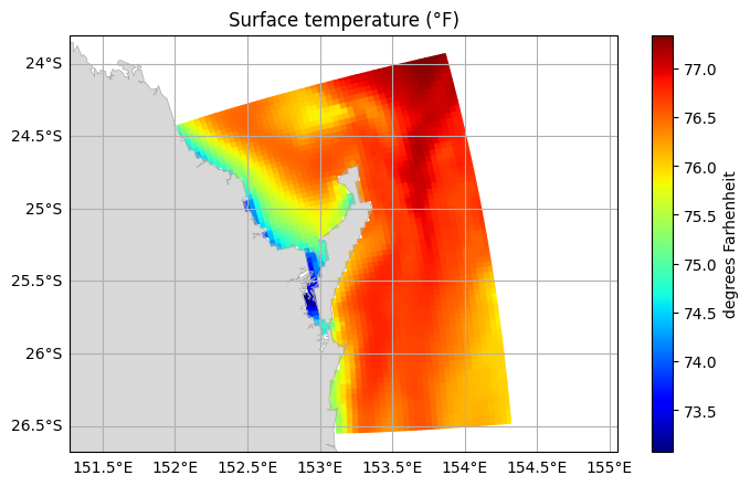
Plotting computed data#
Any data can be plotted on the model grid, as long as the data has the same shape. To demonstrate this, let us make a plot of surface temperature for our American friends.
[11]:
farhenheit_temp = fraser_0['temp'] * 1.8 + 32
farhenheit_temp.attrs.update({
    'long_name': 'Surface temperature (°F)',
    'units': 'degrees Farhenheit'
})
fraser.ems.plot(farhenheit_temp)
Custom plots#
dataset.ems.plot() is useful for making quick plots of your data, but it does not create publication quality plots, and it does not expose any styling options. The following example shows how make a custom plot with your own styling, base layers, and titles. It uses a few tools provided by emsarray to extract the data and construct the polygons, but otherwise does all of the styling manually.
[12]:
import cartopy.crs as ccrs
import cartopy.io.img_tiles as cimgt
import emsarray
import matplotlib.pyplot as plt
import numpy as np
from emsarray.plot import polygon_to_patch, bounds_to_extent
from emsarray.utils import datetime_from_np_time
from matplotlib.collections import PatchCollection
from shapely.geometry import box

# What to plot
dataset = emsarray.tutorial.open_dataset("fraser")
dataset = dataset.isel(time=0, k=-1)
scalar = 'eta'
vector = ('u', 'v')
title = "Sea surface height and surface current velocity"
datetime_stamp = datetime_from_np_time(dataset["time"].values).strftime("%Y-%m-%d %H:%M")

# Constrain the view to this region
view_area = box(152.3, -26.8, 154, -23.5)

# What coordinate reference system the data are in
data_crs = dataset.ems.data_crs

# What coordinate reference system to plot the data in.
# You can choose any projection that you want.
view_crs = ccrs.NearsidePerspective(
    central_longitude=view_area.centroid.x, central_latitude=view_area.centroid.y)

# Set up a figure and some axes, then set view bounds
figure = plt.figure(figsize=(8, 10), dpi=100)
axes = plt.subplot(projection=view_crs)
axes.set_title(title + "\n" + datetime_stamp)
axes.set_aspect(aspect='equal', adjustable='datalim')
axes.set_extent(bounds_to_extent(view_area.bounds), crs=data_crs)

# Add some grid lines
gridlines = axes.gridlines(draw_labels=True, color=(0.1, 0.1, 0.1, 0.1))
gridlines.top_labels = False
gridlines.right_labels = False

# Add a base image layer
axes.add_image(cimgt.Stamen(style='terrain-background', desired_tile_form='RGBA'), 9)
# axes.add_image(cimgt.Stamen(style='terrain-labels', desired_tile_form='RGBA'), 9)
figure.text(
    0.5, 0, "Map tiles by Stamen Design, under CC BY 3.0. Data by OpenStreetMap, under ODbL.",
    va='bottom', ha='center', fontsize=8)

# Plot the data
patches = dataset.ems.make_patch_collection(scalar, edgecolor='face', cmap='plasma')
axes.add_collection(patches)
figure.colorbar(patches, ax=axes, location='right', label='metres')

quiver = dataset.ems.make_quiver(axes, *vector)
axes.add_collection(quiver)
plt.show()
---------------------------------------------------------------------------
ValueError                                Traceback (most recent call last)
File ~/checkouts/readthedocs.org/user_builds/emsarray/conda/v0.1.0/lib/python3.9/site-packages/IPython/core/formatters.py:339, in BaseFormatter.__call__(self, obj)
    337     pass
    338 else:
--> 339     return printer(obj)
    340 # Finally look for special method names
    341 method = get_real_method(obj, self.print_method)

File ~/checkouts/readthedocs.org/user_builds/emsarray/conda/v0.1.0/lib/python3.9/site-packages/IPython/core/pylabtools.py:151, in print_figure(fig, fmt, bbox_inches, base64, **kwargs)
    148     from matplotlib.backend_bases import FigureCanvasBase
    149     FigureCanvasBase(fig)
--> 151 fig.canvas.print_figure(bytes_io, **kw)
    152 data = bytes_io.getvalue()
    153 if fmt == 'svg':

File ~/checkouts/readthedocs.org/user_builds/emsarray/conda/v0.1.0/lib/python3.9/site-packages/matplotlib/backend_bases.py:2290, in FigureCanvasBase.print_figure(self, filename, dpi, facecolor, edgecolor, orientation, format, bbox_inches, pad_inches, bbox_extra_artists, backend, **kwargs)
   2284     renderer = _get_renderer(
   2285         self.figure,
   2286         functools.partial(
   2287             print_method, orientation=orientation)
   2288     )
   2289     with getattr(renderer, "_draw_disabled", nullcontext)():
-> 2290         self.figure.draw(renderer)
   2292 if bbox_inches:
   2293     if bbox_inches == "tight":

File ~/checkouts/readthedocs.org/user_builds/emsarray/conda/v0.1.0/lib/python3.9/site-packages/matplotlib/artist.py:73, in _finalize_rasterization.<locals>.draw_wrapper(artist, renderer, *args, **kwargs)
     71 @wraps(draw)
     72 def draw_wrapper(artist, renderer, *args, **kwargs):
---> 73     result = draw(artist, renderer, *args, **kwargs)
     74     if renderer._rasterizing:
     75         renderer.stop_rasterizing()

File ~/checkouts/readthedocs.org/user_builds/emsarray/conda/v0.1.0/lib/python3.9/site-packages/matplotlib/artist.py:50, in allow_rasterization.<locals>.draw_wrapper(artist, renderer)
     47     if artist.get_agg_filter() is not None:
     48         renderer.start_filter()
---> 50     return draw(artist, renderer)
     51 finally:
     52     if artist.get_agg_filter() is not None:

File ~/checkouts/readthedocs.org/user_builds/emsarray/conda/v0.1.0/lib/python3.9/site-packages/matplotlib/figure.py:2803, in Figure.draw(self, renderer)
   2800         # ValueError can occur when resizing a window.
   2802 self.patch.draw(renderer)
-> 2803 mimage._draw_list_compositing_images(
   2804     renderer, self, artists, self.suppressComposite)
   2806 for sfig in self.subfigs:
   2807     sfig.draw(renderer)

File ~/checkouts/readthedocs.org/user_builds/emsarray/conda/v0.1.0/lib/python3.9/site-packages/matplotlib/image.py:132, in _draw_list_compositing_images(renderer, parent, artists, suppress_composite)
    130 if not_composite or not has_images:
    131     for a in artists:
--> 132         a.draw(renderer)
    133 else:
    134     # Composite any adjacent images together
    135     image_group = []

File ~/checkouts/readthedocs.org/user_builds/emsarray/conda/v0.1.0/lib/python3.9/site-packages/matplotlib/artist.py:50, in allow_rasterization.<locals>.draw_wrapper(artist, renderer)
     47     if artist.get_agg_filter() is not None:
     48         renderer.start_filter()
---> 50     return draw(artist, renderer)
     51 finally:
     52     if artist.get_agg_filter() is not None:

File ~/checkouts/readthedocs.org/user_builds/emsarray/conda/v0.1.0/lib/python3.9/site-packages/cartopy/mpl/geoaxes.py:553, in GeoAxes.draw(self, renderer, **kwargs)
    550     for factory, factory_args, factory_kwargs in self.img_factories:
    551         img, extent, origin = factory.image_for_domain(
    552             self._get_extent_geom(factory.crs), factory_args[0])
--> 553         self.imshow(img, extent=extent, origin=origin,
    554                     transform=factory.crs, *factory_args[1:],
    555                     **factory_kwargs)
    556 self._done_img_factory = True
    558 return matplotlib.axes.Axes.draw(self, renderer=renderer, **kwargs)

File ~/checkouts/readthedocs.org/user_builds/emsarray/conda/v0.1.0/lib/python3.9/site-packages/cartopy/mpl/geoaxes.py:318, in _add_transform.<locals>.wrapper(self, *args, **kwargs)
    313     raise ValueError(f'Invalid transform: Spherical {func.__name__} '
    314                      'is not supported - consider using '
    315                      'PlateCarree/RotatedPole.')
    317 kwargs['transform'] = transform
--> 318 return func(self, *args, **kwargs)

File ~/checkouts/readthedocs.org/user_builds/emsarray/conda/v0.1.0/lib/python3.9/site-packages/cartopy/mpl/geoaxes.py:1374, in GeoAxes.imshow(self, img, *args, **kwargs)
   1370 regrid_shape = self._regrid_shape_aspect(regrid_shape,
   1371                                          target_extent)
   1372 # Lazy import because scipy/pykdtree in img_transform are only
   1373 # optional dependencies
-> 1374 from cartopy.img_transform import warp_array
   1375 original_extent = extent
   1376 img, extent = warp_array(img,
   1377                          source_proj=transform,
   1378                          source_extent=original_extent,
   (...)
   1382                          mask_extrapolated=True,
   1383                          )

File ~/checkouts/readthedocs.org/user_builds/emsarray/conda/v0.1.0/lib/python3.9/site-packages/cartopy/img_transform.py:14, in <module>
     12 import numpy as np
     13 try:
---> 14     import pykdtree.kdtree
     15     _is_pykdtree = True
     16 except ImportError:

File pykdtree/kdtree.pyx:1, in init pykdtree.kdtree()

ValueError: numpy.ndarray size changed, may indicate binary incompatibility. Expected 96 from C header, got 88 from PyObject
<Figure size 800x1000 with 2 Axes>